Build an hourly THHN_1 waterfall

This example answers a concrete plant-floor question:

Pregunta real de plantaReal plant question

How did the THHN_1 sensor rise or fall hour by hour, from its starting value to its final value?

FuenteSource

robotic.sensor_data

TiempoTime

hour · hourly average

MétricaMetric

SUM(aporte)

RangoRange

24 hours through the latest reading

A waterfall is useful when you want more than the sensor level. It explains the journey: where the value rose, where it fell, and where it ended.

What we will build

The original table stores one column per sensor. We will first use SQL Lab to produce four chart-friendly columns:

Column	Meaning
hora	Start of each hourly block.
sensor	Readable sensor name: THHN_1.
valor	Average THHN_1 reading during that hour.
aporte	Change from the previous hour. The first row uses the starting value.

Because of that final rule, adding all contributions takes the waterfall from the starting value to the final value.

1. Prepare the changes in SQL Lab

1. Open SQL Lab.
2. Select Aurora MySQL (Data API) and the robotic schema.
3. Paste and run this query:

SELECT
  actual.hora,
  'THHN_1' AS sensor,
  actual.valor,
  CASE
    WHEN anterior.valor IS NULL THEN actual.valor
    ELSE actual.valor - anterior.valor
  END AS aporte
FROM (
  SELECT
    FROM_UNIXTIME(
      FLOOR(UNIX_TIMESTAMP(`timestamp`) / 3600) * 3600
    ) AS hora,
    AVG(`THHN_1`) AS valor
  FROM `robotic`.`sensor_data`
  WHERE `timestamp` >= (
    SELECT DATE_SUB(MAX(`timestamp`), INTERVAL 24 HOUR)
    FROM `robotic`.`sensor_data`
  )
    AND `THHN_1` IS NOT NULL
  GROUP BY hora
) AS actual
LEFT JOIN (
  SELECT
    FROM_UNIXTIME(
      FLOOR(UNIX_TIMESTAMP(`timestamp`) / 3600) * 3600
    ) AS hora,
    AVG(`THHN_1`) AS valor
  FROM `robotic`.`sensor_data`
  WHERE `timestamp` >= (
    SELECT DATE_SUB(MAX(`timestamp`), INTERVAL 24 HOUR)
    FROM `robotic`.`sensor_data`
  )
    AND `THHN_1` IS NOT NULL
  GROUP BY hora
) AS anterior
  ON anterior.hora = DATE_SUB(actual.hora, INTERVAL 1 HOUR)
ORDER BY actual.hora;

The query returned hour, sensor, value, and contribution, so it is ready to become a chart source.

The 24 hours follow the data

The period ends at the table’s latest timestamp, not necessarily at the current clock time. This also makes the example work with historical data.

2. Check the result before charting

Do not continue until you confirm that:

• there is one row for every expected hour;
• hora is in ascending order;
• valor and aporte contain numbers;
• the first row uses its own valor as aporte;
• later rows calculate current value − previous value.

Watch for gaps

This query compares exact consecutive hours. If an hour is missing, the following row behaves as a new starting point. Check continuity before interpreting the waterfall.

3. Save the virtual source

From the SQL Lab results, save the query as a virtual dataset. A clear name for this example is:

robotic.cascada_THHN_1

This keeps the SQL preparation in one place and lets the Explore screen focus on the visualization.

4. Configure the waterfall

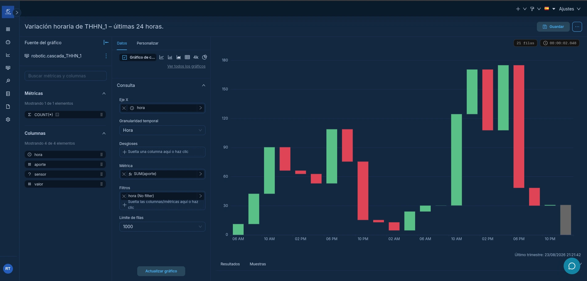
Open the saved dataset and choose Waterfall chart. Set:

Control	Value
X axis	hora
Time grain	Hour
Metric	SUM(aporte)
Row limit	1000

Select Update chart and wait until both the bars and row count appear.

Finished example: each bar explains one hour's change, while the last bar summarizes the final value.

5. Read the result in plain language

• Green: THHN_1 increased from the previous hour.
• Red: THHN_1 decreased.
• Bar height: size of the change, not that hour’s absolute reading.
• Final gray bar: the value reached after accumulating every change.

The screenshot shows a sequence of increases and decreases, with especially large moves during the afternoon section. Hover over a bar for an exact hourly figure; do not estimate it from height alone.

Color does not judge the process

Green means “rose” and red means “fell.” You still need THHN_1’s operating limits to decide whether a change was good, bad, or expected.

✓

Resultado esperadoExpected result

You can tell THHN_1’s complete story: the starting point, every hourly change, and the final value, without confusing changes with absolute readings.

After validating the result, continue to save the chart and add it to a dashboard.